1.2.1 State the fundamental units in the SI system.
|
Mass
Length Time Substance amount Electrical current Thermodynamic temperature Luminosity |
Kilogram
Meter Second Mole Ampere Kelvin Candela |
kg
m s mol A K cd |
1.2.2 Distinguish between fundamental and derived units and give examples of derived units.
Fundamental units are the original SI units, while derived units are new units created from fundamental units.
|
Energy
Force Frequency Pressure Power Voltage Resistance |
Joule
Newton Hertz Pascal Watt Volt Ohm |
J
N Hz Pa W V Ω |
kg × m^2 / s^2
kg × m / s^2 1 / s kg / m / s^2 kg × m^2 / s^3 kg × m^2 / s^3 / A kg × m^2 / s^3 / A^2 |
1.2.3 Convert between different units of quantities.
Questions should always be double-checked in order to make sure that the answer corresponds with the requested units. Common conversions include joules to kilowatts per hour and joules to electron volts. Sometimes numbers need to be multiplied by constants -- for example, the electron volt is equal to 1.60 × 10^-19 joules.
Practice questions
In an unidentified question, an answer is given in joules per second. The question requires a kilowatts per hour value. Which conversions should be made?
Answer: The joules per second value should be multiplied by 3600 to get watts per hour. This value can then be divided by 1000 to get kilowatts per hour.
1.2.4 State units in the accepted SI format.
The IB requires that students write "m × s^-1" instead of "m/s" for all units. This is mentioned in the syllabus:

1.2.5 State values in scientific notation and in multiples of units with appropriate prefixes.
|
Prefix
exa peta tera giga mega kilo hecto deka -- deci centi milli micro nano pico femto atto |
Symbol
E P T G M k h da -- d c m µ n p f a |
Scientific Notation
10^18 10^15 10^12 10^9 10^6 10^3 10^2 10^1 0 10^-1 10^-2 10^-3 10^-6 10^-9 10^-12 10^-15 10^-18 |
(This is given in your formula booklet.)
1.2.6 Describe and give examples of random and systematic errors.
Random errors are errors that occur irregularly and cannot be attributed to a consistent failure in method or equipment. Systematic errors are continuous errors that have a source, such as a broken instrument.
|
Random
|
Systematic
|
1.2.7 Distinguish between precision and accuracy.
1.2.8 Explain how the effects of random errors may be reduced.
Random errors can be reduced through multiple trials of the same experiment. This allows for a better elimination of outliers due to random errors. Repeated experimentation will not change systematic errors as they persist throughout every trial and continuously produce imprecise results.
1.2.9 Calculate quantities and results of calculations to the appropriate number of significant figures.
When giving answers to questions on the exam, answers should always be given with the same amount of significant figures as the smallest amount in the question. For example, if the question contained the numbers 200.345, 600 and 0.2, the answer should be given to one significant figure because 0.2 has the smallest amount of significant figures. Usually, the significant figure amount will remain constant throughout a question. Also note that this is only required when multiplication and division is involved. If the question only asks for the addition of 0.2 and 0.45, the answer should be given as 0.65 regardless of the fact that 0.2 has one significant figure.
1.2.10 State uncertainties as absolute, fractional and percentage uncertainties.
Uncertainties are presented as the tenth of the smallest decimal of a given number. For example:
13.21 m ± 0.01
0.002 g ± 0.001
1.2 s ± 0.1
12 V ± 1
These are called absolute uncertainties. Uncertainties can also be presented as fractional uncertainties, where the tenth of the smallest decimal is presented as a fraction of the original number. For example:
1.2 s ± 0.1
0.1 / 1.2 = 0.0625
Percentage uncertainties are fractional uncertainties converted to percentages:
1.2 s ± 0.1
0.1 / 1.2 x 100 = 6.25 %
1.2.11 Determine the uncertainties in results.
|
Adding/subtracting numbers with uncertainties
|
Multiplying/dividing numbers with uncertainties
|
Functions with uncertainties
- The value should be calculated with the highest possible components and lowest possible components then compared to find the uncertainty of the answer.
- For example: "Calculate the area of a field with a length of 12 ± 1 m and width of 7 ± 0.2 m."
- The 'best value' would be to take 12 and 7 and calculate the area. The highest value uses 13 and 7.2 and the lowest value uses 11 and 6.8. When we work these areas out, we get 84, 93.6 and 74.8. When rounding to the appropriate number of significant figures, we get 84, 94 and 75. This translates to approximately 84 ± 10 m^2.
1.2.12 Identify uncertainties as error bars in graphs.
- The length of the error bars represents the uncertainty range for each value.
1.2.13 State random uncertainty as an uncertainty range (±) and represent it graphically as an error bar.
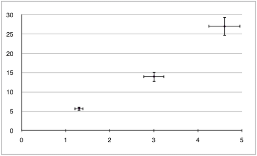
- The uncertainty range is the "± ..." value (ie. 2 ± 0.1). This value can be directly drawn onto a graph at each point as an error bar, as shown in the image above.
- When drawing graphs for the IA, error bars only need to be included if the uncertainty is significant. If they are not included, the student should provide an explanation. If there is a large amount of data, only the largest data point, smallest data point and a few points in-between require error bars.
- Error bars are not required for logarithmic or trigonometric functions.
1.2.14 Determine the uncertainties in the gradient and intercepts of a straight-line graph.
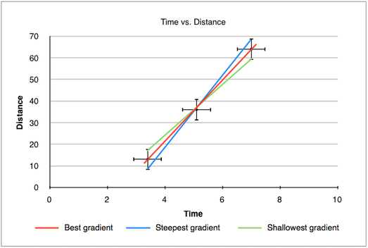
Calculating the uncertainty range of the best-fit line/gradient requires the "largest" (steepest) gradient and "smallest" (shallowest) gradient. The steepest gradient is drawn from the lowest possible value (bottom error bar) to the highest possible value (top error bar). The shallowest gradient is drawn from the largest value to the smallest value. These two gradients are then calculated and compared to the best-fit line. If, for example, the best-fit has a gradient of 9.0, the gradient of the steepest line is 9.2 and the gradient of the shallowest line is 8.8, the best-fit line can be written as 9.0 ± 0.2. The following graph shows how the gradients are drawn:
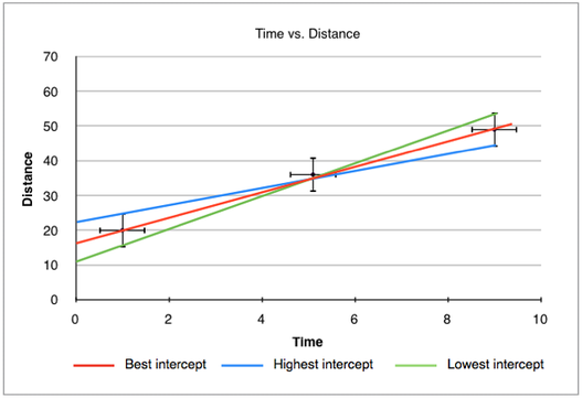
The same method can be applied to the y-intercept. In this case, we check the highest and lowest possible value of the intercept in relation to the steepest and shallowest gradients. In the graph below, the highest intercept is around 23 while the lowest is around 11. If the 'best' intercept is around 17, the overall y-intercept can be written as 17 ± 6.